
Periodic Analysis of the Relationship between Gold, Crude Oil, Exchange Rate and India’s Stock Market
Dr. Anil Kumar Kanungo1*  and Puneet Dang2
1Department of Economics, Lal Bahadur Shastri Institute of Management (LBSIM), New Delhi, India .
2Marsh, and McLennan, India .
http://dx.doi.org/10.12944/JBSFM.02.01-02.05
Copy the following to cite this article:
Kanungo A. K, Dang P. (2021) "Periodic Analysis of the Relationship between Gold, Crude Oil, Exchange Rate and India’s Stock Market". Journal of Business Strategy Finance and Management, 2(1,2). DOI:http://dx.doi.org/10.12944/JBSFM.02.01-02.05
Copy the following to cite this URL:
Kanungo A. K, Dang P. (2021) "Periodic Analysis of the Relationship between Gold, Crude Oil, Exchange Rate and India’s Stock Market". Journal of Business Strategy Finance and Management, 2(1,2). Available From: https://bit.ly/3x0MAYl
Download article (pdf) Citation Manager Publish History


Introduction
Integration of financial markets with the world economy has been a prominent feature of the 21st century. This was evident in early years of 21st century when the stock market, real estate and the commodity market were showing signs of recovery after the Asian Financial crisis during late 1990s.
World economy felt a faster integration of markets can take place through interaction of commodity markets, stock markets and exchange rate. Looking at broadly the growth of the world economy through these instruments, Indian market too aspired to be somewhat more integrated with the world economy.
Investors in Indian economy showed signs of encouragement and went on investing in commodity markets and financial markets assuming these are currently safe routes to multiply their assets and in turn help the Indian economy to integrate and grow.
With the advent of global financial crisis in 2007-08 their hopes were dashed. With the recessionary trends and apprehensions in the economy, investors were forced to detach themselves temporarily from such activities and withdrew their capital from the respective stock markets and started investing in the safe haven i.e. gold or other alternative investments.
This has led to an upsurge in the gold price for the past few months. As per the current scenario gold prices are showing an uptrend with increased tensions globally and central banks investing progressively in it. Thus, the safe-haven’s appeal seems to be increased which is one of the reasons for choosing it as a commodity for the study.
Other important commodity that has experienced a spill over effect of these tensions is crude oil. As the global demand tends to fall with recessionary fears and emerging trade war talks, crude oil prices can be seen going south. Another important factor for the same can be observed as the increased tensions in the middle east. Also, if we trace back the exchange rate prices along with Gold and Crude oil prices, we get a reasonable evidence that shows that these prices are affected by the movement of each other. Thus, this research is carried out to study the reasons for this and the extent of this affect.
Since Gold and crude oil are the most traded commodities in the commodity markets worldwide, thus this study can help in explaining their interrelatedness by studying the movement in their prices and volume. Crude oil being the prominent source of energy globally has a huge demand and hence the ability to impact exchange rates. Moreover, India’s imports have a major concentration of gold and crude oil in its portfolio. Since most of the trades are done in USD, hence this calls for a research to study their interdependencies. Even though the Bretton Woods system has subsided, and a Flexible exchange rate system is applicable in the current scenario, still economies prefer keeping some amount of gold reserves with them. Since in the modern world, all the markets are becoming linked and have spill over effects on each other, hence it is important to study the co-integration and causation of these highly traded commodities, exchange rates and their impact on the stock market. The fluctuations in exchange rate can be observed to have its effects in India due to international trade and a spill over effect on the stock market because of the hopes of increase and/or decrease in profits of companies. Also, the changes in crude oil prices directly impact the companies as they affect the transportation cost. This leads to inflation in an economy and investors prefer buying gold during inflationary times which leads to rise in gold prices as well. Thus, we can clearly say that crude oil and gold have become economic indicators and such a study of their relationship with exchange rate and stock markets can help in forecasting the short-term movements in the currency as well as stock markets. Moreover, to study the impact of these variables on India’s stock market Nifty 50 has been used as a proxy for market. Hence, the research is important as it can help in explaining the relation between India’s exchange rate, gold and crude oil prices, and their impact on India’s stock market.
Review of Literature
While conducting review of literature interesting observations were made. The paper by P?nar Kaya, Bülent Guloglu (2018) explained the forecasting of risk of six commodities viz. crude oil, copper, silver, gold, platinum and palladium for the period 2002-2016 with the help of volatility, VaR, and expected shortfall as risk measures. The researchers showed the squared returns of these six commodities have a significant long memory, volatility, VaR (value at risk) and expected shortfall as per GARCH models. The forecast performance of volatility models and backtest for VaR indicated FIAPARCH model outperforms other GARCH models. Also, volatility, VaR and expected shortfall estimates based on FIAPARCH showed that volatility and market risk of oil is much higher than other commodities. Which casted a doubt on oil being used as a hedging tool. The paper also cites that there has been a rising financialization of commodity markets. Since gold is considered as a safe asset and is used for hedging portfolios across the world, thus it was important to study the volatility and VaR when investments were made in gold assets. Similarly, the article by Ahmad Monir Abdullah and Abul Mansur Mohammad Masih (2016) explains the value addition to the existing research on testing ‘timevarying’ and ‘scale dependent’ volatilities of correlations of the commodities like gold and crude oil. They used daily data of seven commodities and found out that there exists a theoretical relationship between sample commodities. Crude oil, gas, gold and copper variables led the other commodities as shown in their Vector Error-correlation models. They found out that the gas returns were less correlated with the crude oil returns in the short term as shown in their wavelet transform analysis but due to its high volatility it offsets its benefit of diversification in the long run and that an investor holding crude oil can gain by including corn in his portfolio as shown in their Dynamic conditional correlations analysis.
In another article written by Jiancheng Shen, Mohammad Najand and Feng Dong, Wu He (2017) it is observed that Emotions play an important role in both institutional and individual investors’ decision-making process. The authors made an effort to assess the monetary value of emotions. They tried to bridge the gap about how investors’ emotions affect commodity market returns. The purpose of this paper is to investigate whether media-based emotions can be used to predict future commodity returns. The authors examine the short-term predictive power of media-based emotion indices on the following five days’ commodity returns. The research adopts a proprietary data set of commodity-specific market emotions, which is computed based on a comprehensive textual analysis of sources from newswires, internet news sources and social media.
The paper by Mongi Arfaoui and Aymen Ben Rejeb (2017) examined the oil, gold, US dollar and stock prices interdependencies in a global perspective and identified instantaneously direct and indirect linkages among them. A methodology based on simultaneous equations system was used to identify direct and indirect linkages for the period 1995-2015. The results show significant interactions between all markets. The authors found a negative relation between oil and stock prices, but oil price is significantly and positively affected by gold and USD. Oil price is also affected by oil futures prices and by Chinese oil gross imports. Gold rate is concerned by changes in oil, USD and stock markets. The US dollar is negatively affected by stock market and significantly by oil and gold price.
Another study by Wei Fan, Sihai Fang and Tao Lu (2014) has identified what macro factors affect the gold prices and how they impact on the gold price. An EGARCH model is applied to test the volatility of gold price. A VAR method is applied to validate the idea by decomposing gold’s value into three parts according to its features. The research found out that three macro-factors have significant impact on the gold’s price.
Semei Coronado, Rebeca Jiménez-Rodríguez, and Omar Rojas (2018) in a study have explained the results of the linear Granger causality tests to show that the stock market causes the two commodity markets, but not vice versa, and that there is a significant unilateral linear Granger causality running from the crude oil market to the gold market.
After analysing certain amount of review of literature, it was observed that no serious evidence was found to understand the causation of price changes amongst the exchange rate influencing the prices of gold and crude oil or is it vice-versa? It was further noticed that the general perception about change in exchange rate sometimes influence gold and oil prices may not be true. The gaps that emerged after going through literature are whether price of exchange rate really impact the long term and the short-term relationship between exchange rate, gold and price of oil. The research paper makes an attempt to study such dimensions in detail by employing various econometric models.
Research Objectives
The specific objectives of this paper are to understand the causation of price changes amongst the exchange rate influencing the prices of gold and crude oil or is it vice-versa? Secondly, it makes an attempt to find if there exists a cointegration between the three variables, i.e. gold, crude oil and Dollar-Rupee exchange rate. Thirdly, it proposes to study the long-term and short-term relation between exchange rate, gold and crude oil prices. Lastly it aims to study if there’s a spill over effect on India’s stock market.
Hypotheses
The paper aims to test the following hypotheses.
The variables used in the study are ‘dollar-rupee exchange rate’, ‘price of gold’, and ‘price of crude oil (WTI)’.
H1: There is no cointegration (long-run relationship) amongst the three variables.
H2: There is no cause-and-effect relationship amongst the three variables.
H3: There is no effect of the three variables on Indian stock market.
Research Methodology
The study further follows a robust research methodology.
Data Collection: The daily spot prices have been taken for gold and crude oil traded on MCX. Also, for the dollar-rupee exchange rate data daily spot prices have been taken.
Data Source: Bloomberg.
Time Period: Time period used for the study is from January 2005 to December 2019.
Tools and Techniques
As the study involves time series analysis, econometrics techniques are being applied. Data preparation have been done on Microsoft Excel and Eviews 10.0 would be used as an analytical tool for the study. The study employs Granger causality test, Johansen’s Cointegration, and Vector Autoregression on the data, which are divided into three phases, viz. Pre-crisis (2005-2007), crisis (2007-2009) and Post-crisis (2009-2019). To study the spill over effect on India’s stock market regression analysis has been used.
Research Analysis
Unit Root Test (ADF)
Before finding out the cointegration between the variables viz. Gold, Crude Oil and Dollar-Rupee Exchange rate, it was important to confirm if these series are non-stationary at level form i.e. raw data. Hence, ADF test was used to confirm the non-stationarity at level form and the data was also checked at Integrated order 1 i.e. I(1) to see if the data is stationary at I(1) or not. The spot prices of Gold, Crude Oil and Dollar-Rupee exchange rate were used for the pre-crisis period, i.e. 10/24/2005 to 7/31/2007, for the crisis period, i.e. 8/02/2007 to 6/30/2009 and for the post-crisis period, i.e. 7/02/2009 to 1/31/2020 and tested using ADF (Augmented Dickey Fuller Test) for all the three cases viz. without drift, with drift, and with drift and trend. The same test was repeated on the first difference i.e. I (1) of these variables.
Table 1: ADF Test Results (Spot Prices)
|
Pre-Crisis Period |
||||||
|
Variable |
Without drift |
With drift |
With drift and trend |
|||
|
t-stat |
Probability |
t-stat |
Probability |
t-stat |
Probability |
|
|
Gold |
0.607918 |
0.8473 |
-2.730707 |
0.0697 |
-2.242270 |
0.4643 |
|
Crude Oil |
0.174240 |
0.7364 |
-1.815099 |
0.3730 |
-1.792074 |
0.7072 |
|
USD/INR |
-1.632055 |
0.0969 |
0.706632 |
0.9922 |
-0.965709 |
0.9461 |
|
Crisis Period |
||||||
|
Variable |
Without drift |
With drift |
With drift and trend |
|||
|
t-stat |
Probability |
t-stat |
Probability |
t-stat |
Probability |
|
|
Gold |
1.132838 |
0.9337 |
-1.642168 |
0.4601 |
-2.977954 |
0.1396 |
|
Crude Oil |
-0.251920 |
0.5951 |
-1.165920 |
0.6904 |
-1.402409 |
0.8593 |
|
USD/INR |
1.241361 |
0.9456 |
-0.647334 |
0.8569 |
-1.626816 |
0.7811 |
|
Post-Crisis Period |
||||||
|
Variable |
Without drift |
With drift |
With drift and trend |
|||
|
|
t-stat |
Probability |
t-stat |
Probability |
t-stat |
Probability |
|
Gold |
2.020502 |
0.9901 |
-1.057747 |
0.7343 |
-1.803657 |
0.7030 |
|
Crude Oil |
-0.395010 |
0.5418 |
-1.987211 |
0.2927 |
-2.118645 |
0.5345 |
|
USD/INR |
1.675165 |
0.9776 |
-0.643031 |
0.8585 |
-2.349345 |
0.4064 |
From the ADF tests performed on the spot prices it could be observed that the p-value is greater than 5% for all the three variables viz. “Gold”, “Crude Oil” and “USD/INR” at their level form in all the three time periods. This was true for all the three cases namely “without drift”, “with drift”, and “with drift and trend”. Thus, we can say that unit root exists in the time series data for all the three variables during all the three time periods.
Hence, we can say that the data is non-stationary at level form. Non-stationarity implies that the data has its mean values, variance values and covariance values that change over a period.
Since using non-stationary time series data may lead to spurious results, hence the data was checked for stationarity on its first difference i.e. of integrated order 1.
Table 2: ADF Test Results (First Difference)
|
|
Pre-Crisis |
Crisis |
Post-Crisis |
|||
|
Variable |
Without drift |
|||||
|
t-stat |
Probability |
t-stat |
Probability |
t-stat |
Probability |
|
|
D(Gold) |
-21.08836 |
0.0000 |
-21.13286 |
0.0000 |
-48.74382 |
0.0001 |
|
D(Crude Oil) |
-21.51291 |
0.0000 |
-22.99684 |
0.0000 |
-52.02260 |
0.0001 |
|
D(USD/INR) |
-20.10868 |
0.0000 |
-19.12993 |
0.0000 |
-38.17781 |
0.0000 |
Since the p-value is less than 5% thus, we can say that the Gold, Crude Oil and USD/INR spot rates are stationary at first difference or stationary at I(1) for all the three time periods, viz. Pre-Crisis, Crisis and Post Crisis.
Now, since we know that all the three variables contain unit root at level form and are stationary at I(1) we can perform our causality test viz. Granger Causality test to study the relation amongst the three.
Granger Causality Test
Lag Selection - Using the VAR lag length selection criteria test for the endogenous variables Gold, USD/INR and Crude Oil for the per-crisis period we got the following results.
Table 3: Observations Included.
| Pre-Crisis: 421 | |||
| Crisis: 445 | |||
| Post Crisis: 2477 | |||
|
|
Pre-Crisis Period |
Crisis Period |
Post Crisis Period |
|
Lag |
AIC |
AIC |
AIC |
|
0 |
33.84876 |
39.06061 |
42.67732 |
|
1 |
21.91834 |
26.04357 |
25.62432 |
|
2 |
21.81485* |
25.95941 |
25.61164 |
|
3 |
21.84620 |
25.93580* |
25.60692 |
|
4 |
- |
25.96000 |
25.59822 |
|
5 |
- |
- |
25.59812* |
|
6 |
- |
- |
25.60081 |
Using the Akaike Information Criterion (AIC), we can observe that the optimal lag order is of 2 for Pre-Crisis period, 3 for Crisis Period and 5 for Post-Crisis period.
Hence, the granger causality tests have been performed with the lag structures mentioned above for these time periods.
Granger Causality Test results
The granger causality test has been performed using the variables at their first difference in order to nullify the effect of drift and trend in the data. Moreover, Causality tests using the variable data at level form can show spurious results.
Hypothesis: The null hypothesis for granger causality test is that there exists no cause and effect relationship amongst the variables.
Thus, if the value is less than 5% we reject the null hypothesis and if the value is more than 95% we fail to reject the null hypothesis.
Table 4: Pairwise Granger Causality Tests.
|
Null Hypothesis |
Pre-Crisis Period |
Crisis Period |
Post-Crisis Period |
|||
|
Probability Value |
Reject / Fail to reject |
Probability Value |
Reject / Fail to reject |
Probability Value |
Reject / Fail to reject |
|
|
D(USDINR) does not Granger Cause D(GOLD) |
0.8801 |
Fail to reject |
0.1817 |
Fail to reject |
0.2979 |
Fail to reject |
|
D(GOLD) does not Granger Cause D(USDINR) |
0.0125 |
Reject |
0.5385 |
Fail to reject |
3.E-05 |
Reject |
|
D(WTI) does not Granger Cause D(GOLD) |
1.E-11 |
Reject |
2.E-09 |
Reject |
9.E-05 |
Reject |
|
D(GOLD) does not Granger Cause D(WTI) |
0.5525 |
Fail to reject |
0.0024 |
Reject |
0.0019 |
Reject |
|
D(WTI) does not Granger Cause D(USDINR) |
0.7498 |
Fail to reject |
0.1994 |
Fail to reject |
0.0632 |
Fail to reject |
|
D(USDINR) does not Granger Cause D(WTI) |
0.8630 |
Fail to reject |
0.1114 |
Fail to reject |
0.0010 |
Reject |
Hence, from the above anlysis mentioned in the table, it can be inferred that through the Granger causality test it is proven that, “Gold” complies with granger cause in “USD/INR”. Similarly “Crude oil” also does granger cause “Gold” in the pre-crisis period as the p-values are less than 5 per cent.
Since the p-values for the other tests were higher than 5per cent, we were unable to reject the null hypothesis for those tests. Hence, we can infer that, “USD/INR” doesn’t granger cause “Gold”, “Gold” does not granger cause “Crude Oil”, “Crude Oil” does not granger cause “USD/INR”, and “USD/INR” does not granger cause “Crude Oil”.
For the crisis period, it can be stated that “Crude Oil” does Granger cause “Gold” and “Gold” does granger cause “Crude oil” prices. Thus, there exists a two-way relationship between “Gold” and “Crude oil”. There is no direct causality relation between “USD/INR” and “Gold” and “Crude Oil” and “USDINR”.
From the above table it can be observed that, “Gold” does granger cause “USDINR”, “Crude oil” does granger cause “Gold”, “Gold” does granger cause “Crude oil” and “USDINR” does granger cause “Crude Oil” for the post crisis period.
Thus, in the current scenario, the causality amongst the variables has increased and it is evident from the data. We can observe from the above-mentioned granger causality tests that the three variables have a spillover effect over one another. This wasn’t much prevalent in the pre-crisis and crisis periods.
Johansen’s Cointegration Test
Johansen’s Cointegration test was applied to analyse if these three variables form a cointegrating relationship. It was observed that the spot prices of the three variables show a linear deterministic trend. Thus, Johansen’s cointegration test was performed with a lag interval of 2 to check for the presence of cointegration. The table shows the Eigenvalues, Trace statistic values and probability values for lag 0, lag 1 and lag 2 for the three variables i.e. “Gold”, “USD/INR” and “Crude Oil”.
For the Johannsen’s Cointegration test, our hypothesis is that there exists no cointegration amongst the variables. Thus, if the probability value comes out to be less than 5%, we reject the null hypothesis else we fail to reject the null hypothesis. Here, we can observe that the probability value at ‘None’ is 67.64% at ‘Atmost 1’ is 67.64% and at ‘Atmost 2’ is 35.45% for the Pre-Crisis period, the probability value at ‘None’ is 51.39% at ‘Atmost 1’ is 58.58% and at ‘Atmost 2’ is 38.22% for the Crisis Period and the probability value at ‘None’ is 70.69% at ‘Atmost 1’ is 75.65% and at ‘Atmost 2’ is 62.97% for the Post-Crisis Period.
*Here none, atmost1 and atmost 2 refer to the number of cointegrating relationships.
Since, all the values are greater than 5% level thus we fail to reject the null hypothesis. Which means that there exists no cointegration amongst the variables.
VAR – The results for VAR at first differences of Gold, USDINR and Crude oil i.e. after making the data stationary are shown below.
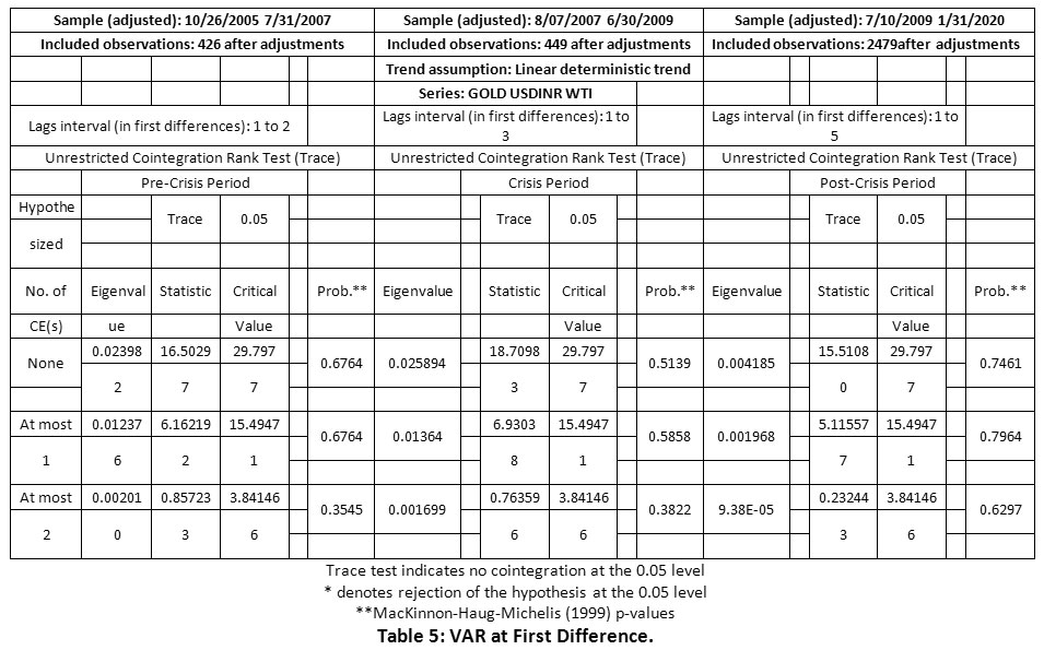 |
Table 5: VAR at First Difference. Click here to view Table |
Table 6: Vector Autoregression Estimates.
|
Date: 02/13/20 Time: 13:55 |
|||
|
Sample (adjusted): 10/26/2005 7/31/2007 |
|||
|
Included observations: 426 after adjustments |
|||
|
Standard errors in ( ) & t-statistics in [ ] |
|||
|
|
D(GOLD) |
D(USDINR) |
D(WTI) |
|
|
|
|
|
|
D(GOLD(-1)) |
-0.059085 |
0.000208 |
0.023518 |
|
|
(0.04923) |
(6.4E-05) |
(0.02566) |
|
|
[-1.20008] |
[ 3.24132] |
[ 0.91664] |
|
|
|
|
|
|
D(GOLD(-2)) |
-0.009311 |
4.24E-05 |
0.014627 |
|
|
(0.04673) |
(6.1E-05) |
(0.02435) |
|
|
[-0.19927] |
[ 0.69664] |
[ 0.60069] |
|
|
|
|
|
|
D(USDINR(-1)) |
-67.22675 |
0.035483 |
-10.07880 |
|
|
(38.0728) |
(0.04955) |
(19.8404) |
|
|
[-1.76574] |
[ 0.71604] |
[-0.50799] |
|
|
|
|
|
|
D(USDINR(-2)) |
6.694508 |
-0.023467 |
-0.646842 |
|
|
(37.8473) |
(0.04926) |
(19.7229) |
|
|
[ 0.17688] |
[-0.47637] |
[-0.03280] |
|
|
|
|
|
|
D(WTI(-1)) |
0.711575 |
-0.000137 |
-0.045794 |
|
|
(0.09505) |
(0.00012) |
(0.04953) |
|
|
[ 7.48608] |
[-1.10466] |
[-0.92450] |
|
|
|
|
|
|
D(WTI(-2)) |
0.019111 |
-0.000160 |
-0.070319 |
|
|
(0.10120) |
(0.00013) |
(0.05274) |
|
|
[ 0.18884] |
[-1.21329] |
[-1.33333] |
|
|
|
|
|
|
C |
3.335847 |
-0.011740 |
0.571548 |
|
|
(5.10510) |
(0.00664) |
(2.66036) |
|
|
[ 0.65343] |
[-1.76678] |
[ 0.21484] |
Results
From the above table we can observe that Gold I(1) at a lag of 1 has a weakly endogenous influence on Gold at I(1) as the t-stat stands at -1.20008, which implies that a percent increase in Gold I(1) at lag 1 will lead to a decrease of 5.9085% for the Gold I(1).
From the above table we can observe that Gold I(1) at a lag of 1 has a strongly exogenous influence on USDINR at I(1) as the t-stat stands at 3.24132, which implies that a percent increase in Gold I(1) at lag 1 will lead to a increase of 0.0208% for the USDINR I(1).
From the above table we can observe that USDINR I(1) at a lag of 1 has a strongly exogenous influence on Gold at I(1) as the t-stat stands at -1.76574.
From the above table we can observe that Crude Oil I(1) at a lag of 1 has a strongly exogenous influence on Gold at I(1) as the t-stat stands at 7.48608.
From the above table we can observe that Crude Oil I(1) at a lag of 1 has a strongly exogenous influence on USDINR at I(1) as the t-stat stands at -1.10466
Crisis Period
Table 7: VAR at First Difference.
|
Vector Autoregression Estimates |
|||
|
Date: 02/13/20 Time: 14:51 |
|||
|
Sample (adjusted): 8/07/2007 6/30/2009 |
|||
|
Included observations: 449 after adjustments |
|||
|
Standard errors in ( ) & t-statistics in [ ] |
|||
|
|
D(GOLD) |
D(USDINR) |
D(WTI) |
|
|
|
|
|
|
D (GOLD (-1)) |
-0.028364 |
-5.82E-05 |
0.015435 |
|
|
(0.04844) |
(6.8E-05) |
(0.03006) |
|
|
[-0.58554] |
[-0.85697] |
[ 0.51341] |
|
|
|
|
|
|
D (GOLD (-2)) |
-0.048883 |
-9.06E-05 |
0.089405 |
|
|
(0.04823) |
(6.8E-05) |
(0.02994) |
|
|
[-1.01348] |
[-1.33923] |
[ 2.98653] |
|
|
|
|
|
|
D (GOLD (-3)) |
-0.040202 |
-2.37E-05 |
-0.051152 |
|
|
(0.04683) |
(6.6E-05) |
(0.02907) |
|
|
[-0.85839] |
[-0.36113] |
[-1.75973] |
|
|
|
|
|
|
D (USDINR (-1)) |
-11.67576 |
0.114998 |
-21.66022 |
|
|
(34.9113) |
(0.04896) |
(21.6678) |
|
|
[-0.33444] |
[ 2.34873] |
[-0.99965] |
|
|
|
|
|
|
D (USDINR (-2)) |
78.04982 |
0.040084 |
39.19541 |
|
|
(35.1296) |
(0.04927) |
(21.8033) |
|
|
[ 2.22177] |
[ 0.81360] |
[ 1.79768] |
|
|
|
|
|
|
D (USDINR (-3)) |
-27.72207 |
0.030697 |
5.608919 |
|
|
(35.3511) |
(0.04958) |
(21.9408) |
|
|
[-0.78419] |
[ 0.61917] |
[ 0.25564] |
|
|
|
|
|
|
D (WTI (-1)) |
0.515703 |
0.000238 |
-0.077533 |
|
|
(0.07791) |
(0.00011) |
(0.04836) |
|
|
[ 6.61880] |
[ 2.18030] |
[-1.60331] |
|
|
|
|
|
|
D (WTI (-2)) |
0.104671 |
7.27E-05 |
-0.037967 |
|
|
(0.08056) |
(0.00011) |
(0.05000) |
|
|
[ 1.29922] |
[ 0.64327] |
[-0.75931] |
|
|
|
|
|
|
D (WTI (-3)) |
-0.073427 |
-1.74E-05 |
0.062790 |
|
|
(0.08028) |
(0.00011) |
(0.04983) |
|
|
[-0.91462] |
[-0.15427] |
[ 1.26017] |
|
|
|
|
|
|
C |
13.19692 |
0.015483 |
-0.089535 |
|
|
(9.11067) |
(0.01278) |
(5.65457) |
|
|
[ 1.44851] |
[ 1.21172] |
[-0.01583] |
From the above table we can observe that Gold I(1) at a lag of 2 has a weakly endogenous influence on Gold at I(1) as the t-stat stands at-1.01348, which implies that a percent increase in Gold I(1) at lag 2 will lead to a decrease of 4.8883% for the Gold I(1).
From the above table we can observe that Gold I(1) at a lag of 2 has a weakly exogenous influence on USDINR at I(1) as the t-stat stands at -1.33923.
From the above table we can observe that Gold I(1) at a lag of 2 has a strongly exogenous influence on Crude Oil at I(1) as the t-stat stands at 2.98653, which implies that a percent change in Gold I(1) at lag 2 will lead to a 8.94% increase in crude oil prices.
From the above table we can observe that USDINR I(1) at a lag of 1 has a strongly endogenous influence on USDINR at I(1) as the t-stat stands at 2.34873, which implies that a percent change in Gold I(1) at lag 2 will lead to a 11.49% increase in crude oil prices.
From the above table we can observe that Crude Oil I(1) at a lag of 1 has a strongly exogenous influence on Gold at I(1) as the t-stat stands at 6.6188.
From the above table we can observe that Crude Oil I(1) at a lag of 1 has a strongly exogenous influence on USDINR at I(1) as the t-stat stands at 2.1803.
Post Crisis Period
Table 8: VAR at First Difference.
|
Vector Autoregression Estimates |
|||
|
Date: 02/13/20 Time: 17:30 |
|||
|
Sample (adjusted): 7/10/2009 1/31/2020 |
|||
|
Included observations: 2479 after adjustments |
|||
|
Standard errors in ( ) & t-statistics in [ ] |
|||
|
|
D(GOLD) |
D(USDINR) |
D(WTI) |
|
D(GOLD(-1)) |
0.014059 |
0.000115 |
0.023092 |
|
|
(0.02033) |
(2.4E-05) |
(0.00706) |
|
|
[ 0.69151] |
[ 4.77478] |
[ 3.27154] |
|
|
|
|
|
|
D(GOLD(-2)) |
0.016505 |
2.31E-05 |
0.010128 |
|
|
(0.02046) |
(2.4E-05) |
(0.00710) |
|
|
[ 0.80673] |
[ 0.95235] |
[ 1.42591] |
|
|
|
|
|
|
D(GOLD(-3)) |
0.017723 |
5.39E-06 |
-0.020874 |
|
|
(0.02043) |
(2.4E-05) |
(0.00709) |
|
|
[ 0.86773] |
[ 0.22287] |
[-2.94368] |
|
|
|
|
|
|
D(GOLD(-4)) |
0.021216 |
3.07E-05 |
-0.000782 |
|
|
(0.02046) |
(2.4E-05) |
(0.00710) |
|
|
[ 1.03698] |
[ 1.26705] |
[-0.11008] |
|
|
|
|
|
|
D(GOLD(-5)) |
-0.009581 |
6.72E-06 |
0.002184 |
|
|
(0.02041) |
(2.4E-05) |
(0.00709) |
|
|
[-0.46932] |
[ 0.27827] |
[ 0.30818] |
|
|
|
|
|
|
D(USDINR(-1)) |
11.41104 |
-0.020509 |
-0.682822 |
|
|
(17.2677) |
(0.02043) |
(5.99484) |
|
|
[ 0.66083] |
[-1.00376] |
[-0.11390] |
|
|
|
|
|
|
D(USDINR(-2)) |
-9.579941 |
-0.083013 |
-17.42582 |
|
|
(17.2196) |
(0.02037) |
(5.97815) |
|
|
[-0.55634] |
[-4.07426] |
[-2.91492] |
|
|
|
|
|
|
D(USDINR(-3)) |
-20.51515 |
0.041854 |
19.99730 |
|
|
(17.2497) |
(0.02041) |
(5.98858) |
|
|
[-1.18931] |
[ 2.05063] |
[ 3.33924] |
|
|
|
|
|
|
D(USDINR(-4)) |
-1.107381 |
0.045061 |
5.474914 |
|
|
(17.2436) |
(0.02040) |
(5.98647) |
|
|
[-0.06422] |
[ 2.20854] |
[ 0.91455] |
|
|
|
|
|
|
D(USDINR(-5)) |
38.90466 |
0.041836 |
8.008643 |
|
|
(17.2102) |
(0.02036) |
(5.97489) |
|
|
[ 2.26055] |
[ 2.05444] |
[ 1.34038] |
|
|
|
|
|
|
D(WTI(-1)) |
0.223378 |
3.04E-05 |
-0.045012 |
|
|
(0.05859) |
(6.9E-05) |
(0.02034) |
|
|
[ 3.81236] |
[ 0.43800] |
[-2.21278] |
|
|
|
|
|
|
D(WTI(-2)) |
-0.095046 |
-4.22E-05 |
0.025580 |
|
|
(0.05880) |
(7.0E-05) |
(0.02041) |
|
|
[-1.61648] |
[-0.60668] |
[ 1.25312] |
|
|
|
|
|
|
D(WTI(-3)) |
-0.109026 |
0.000165 |
-0.025463 |
|
|
(0.05862) |
(6.9E-05) |
(0.02035) |
|
|
[-1.85984] |
[ 2.38021] |
[-1.25116] |
|
|
|
|
|
|
D(WTI(-4)) |
0.073136 |
0.000149 |
0.031405 |
|
|
(0.05865) |
(6.9E-05) |
(0.02036) |
|
|
[ 1.24707] |
[ 2.14783] |
[ 1.54247] |
|
|
|
|
|
|
D(WTI(-5)) |
-0.017579 |
-7.82E-05 |
0.008455 |
|
|
(0.05856) |
(6.9E-05) |
(0.02033) |
|
|
[-0.30021] |
[-1.12928] |
[ 0.41594] |
|
|
|
|
|
|
C |
9.733602 |
0.006913 |
0.016598 |
|
|
(4.70105) |
(0.00556) |
(1.63207) |
|
|
[ 2.07051] |
[ 1.24277] |
[ 0.01017] |
From the above table we can observe that Gold I(1) at a lag of 1 has a strongly exogenous influence on USDINR and crude oil at I(1) as the t-stat stands at 4.7747 and 3.2715 respectively.
From the above table we can observe that Gold I(1) at a lag of 4 has a weakly endogenous influence on gold at I(1) as the t-stat stands at 1.0369.
From the above table we can observe that USDINR I(1) at a lag of 1 has a weakly endogenous influence on USDINR at I(1) as the t-stat stands at -1.0037.
From the above table we can observe that USDINR I(1) at a lag of 5 has a strongly exogenous influence on gold at I(1) as the t-stat stands at 2.2605, and a weakly exogenous influence on crude oil as the t-stat value stands at 1.3403.
From the above table we can observe that Crude oil I(1) at a lag of 1 has a strongly exogenous influence on crude oil at I(1) as the t-stat stands at 3.8126 and also a strongly endogenous influence on crude oil as the t-stat value stands at -2.2127.
Impact of Gold, Crude Oil and Dollar-Rupee Exchange Rate on India’s Stock Market
To study the impact of gold, crude oil and USDINR on India’s stock market; NIFTY50 has been used as a proxy for the market.
Why NIFTY50?
NIFTY50 captures the performance of top 50 large-cap companies that are listed on National Stock Exchange (India). NSE makes sure to closely monitor these companies and remove and add new companies as their free-float market cap changes along with time.
Methodology
To study the impact of gold, crude oil and USDINR on India’s stock market, we have used linear regression analysis. The data has been divided into three phases i.e. Pre crisis (2005-2007), Crisis (2007-2009) and Post Crisis (2009-2019). Hence, the linear regression is performed on the data using Ms Excel.
Multiple Linear Regression
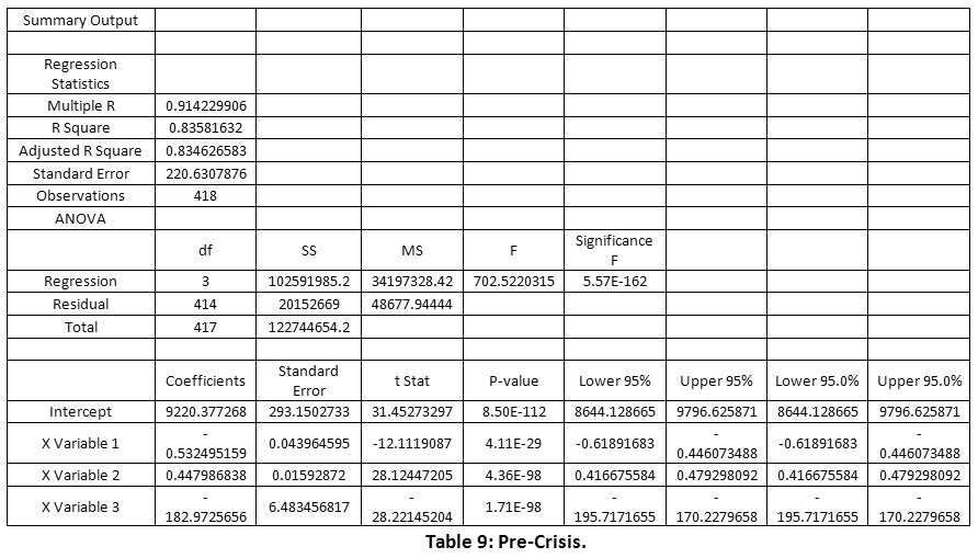 |
Table 9: Pre-Crisis. Click here to view Table |
Regression Equation
Nifty = 9220.37 – 0.532*WTI + 0.447*Gold – 182.973*USDINR
Here, X variable 1 refers to WTI (crude oil), X variable 2 refers to Gold and X variable 3 refers to USDINR.
Analysis
R square and adjusted R square are almost equal thus model is a good fit, moreover, R square value is high which means there is a good accuracy.
One-unit change in WTI prices will bring down Nifty index by 0.532 points. Gold will increase Nifty by 0.44 points and exchange rate will bring down Nifty by 182.973 points.
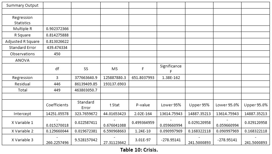 |
Table 10: Crisis. Click here to view Table |
Regression Equation
Nifty = 14251.05578 – 0.0152*WTI + 0.1296*Gold – 260.2257*USDINR
Here, X variable 1 refers to WTI (crude oil), X variable 2 refers to Gold and X variable 3 refers to USDINR.
Analysis
R square and adjusted R square are almost equal thus model is a good fit, moreover, R square value is high which means there is a good accuracy.
One-unit change in WTI prices will bring down Nifty index by 0.0152 points. Gold will increase Nifty by 0.1296 points and exchange rate will bring down Nifty by 260.2257 points.
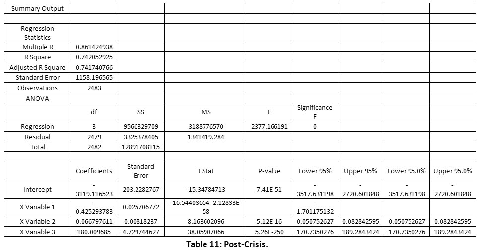 |
Table 11: Post-Crisis?. Click here to view Table |
Regression Equation
Nifty = -3119.116523 – 0.4252*WTI + 0.06679*Gold + 190.0096*USDINR
Here, X variable 1 refers to WTI (crude oil), X variable 2 refers to Gold and X variable 3 refers to USDINR.
Analysis
R square and adjusted R square are almost equal thus model is a good fit, moreover, R square value is high which means there is a good accuracy.
One-unit change in WTI prices will bring down Nifty index by 0.4252 points. Gold will increase Nifty by 0.0667 points and exchange rate will increase Nifty by 180.0096 points.
Research Implications
Practical Implications:
- The findings of this research are vital to various stakeholders and participants of the markets who trade in “Gold”, “Crude Oil”, “USD/INR” and India’s Stock market.
- The results thereof, would also help the importers, exporters, commodity traders, fund managers, corporates and India’s government in framing their policies and strategies.
- Investors and fund managers can use the research findings to understand the relationship of these variables and find cross hedging opportunities.
- Since India is a large importer of crude oil and it directly influences the cost of transportation, and eventually the final price to the consumer, this study can be helpful in furthering new areas of research relating broadly to this study.
- Such research studies can propel the researchers to find out the impact of crude oil prices on India’s inflation.
- Moreover, this study also provides a wider scope to the researchers to remain engaged with the issue of impact of changes in the prices of these variables to India’s inflation rate. Besides, the study provides a direction to look into other commodity variables such as natural gas and silver which can demonstrate similar or differential spill-over effects.
Conclusion
The research study aimed at understanding the relationship amongst the variables, “Gold”, “Crude Oil” and “Dollar-Rupee” exchange rate and finding their impact on India’s stock market. This was important because various financial markets are becoming interrelated and have been observing a contagion effect. Thus, the data for these variables were divided into three periods, i.e. Pre-Crisis, Crisis and Post Crisis and it was analysed using various econometric techniques such as Granger Causality, Johansen’s Cointegration, VAR, and Multiple Linear Regression analysis.
This research study dals with a specialized domain of a financial and commodity market. It adds to the existing body of literature dealing with commodities, foreign exchange rate and stock market. This will help the research community in understanding the relationship so that they can follow up and conduct research on the relationship between the phases carried out in the study to arrive at new dimension emanating in this highly volatile market.
This kind of a study can create a base for other commodity such as silver, base metals and other hard currencies like euro, pound sterling, or even digital currency such as blockchain. Post Covid-19 era could be a relevant phase for future research based on these hypotheses and research analysis.
The paper at the end summarises the following analysis through methodology and techniques.
Granger Causality test was used to find the cause-and-effect relationship between these variables over the three time periods and the results showed that, for Pre-Crisis period “Gold” does granger cause “USD/INR” and “Crude oil” does granger cause “Gold”. No other relationship could be established in the Pre-Crisis period. For the Crisis Period, it was observed that “Crude Oil” does Granger cause “Gold” and “Gold” does granger cause “Crude oil” prices. Thus, there exists a two-way relationship between “Gold” and “Crude oil”.
There is no direct causality relation between “USD/INR” and “Gold” and “Crude Oil” and “USDINR”. For the Post-Crisis period, it was observed that “Gold” does granger cause “USDINR”, “Crude oil” does granger cause “Gold”, “Gold” does granger cause “Crude oil” and “USDINR” does granger cause “Crude Oil”.
Hence, the causality results can help the
Thus, in the current scenario, the causality amongst the variables has increased and it is evident from the data. We can observe from the above-mentioned granger causality tests that the three variables have a spillover effect over one another. This wasn’t much prevalent in the pre-crisis and crisis periods.
From the Johannsen’s Cointegration test results we can observe that the probability values at ‘None’, ‘Atmost 1’ and at ‘Atmost 2’ for the Pre-Crisis period, the Crisis Period and the Post-Crisis Period are significantly high. Here none, atmost1 and atmost 2 refer to the number of cointegrating relationships. Thus, there exists no cointegration amongst the variables.
The results from VAR showed that for the Pre-Crisis period Gold I(1) at a lag of 1 has a weakly endogenous influence on Gold at I(1) as the t-stat stands at -1.20008, which implies that a percent increase in Gold I(1) at lag 1 will lead to a decrease of 5.9085% for the Gold I(1). From the above table we can observe that Gold I(1) at a lag of 1 has a strongly exogenous influence on USDINR at I(1) as the t-stat stands at 3.24132, which implies that a percent increase in Gold I(1) at lag 1 will lead to a increase of 0.0208% for the USDINR I(1). From the above table we can observe that USDINR I(1) at a lag of 1 has a strongly exogenous influence on Gold at I(1) as the t-stat stands at -1.76574. From the above table we can observe that Crude Oil I(1) at a lag of 1 has a strongly exogenous influence on Gold at I(1) as the t-stat stands at 7.48608. From the above table we can observe that Crude Oil I(1) at a lag of 1 has a strongly exogenous influence on USDINR at I(1) as the t-stat stands at -1.10466. For the Crisis period we can observe that Gold I(1) at a lag of 2 has a weakly endogenous influence on Gold at I(1) as the t-stat stands at-1.01348, which implies that a percent increase in Gold I(1) at lag 2 will lead to a decrease of 4.8883% for the Gold I(1). From the above table we can observe that Gold I(1) at a lag of 2 has a weakly exogenous influence on USDINR at I(1) as the t-stat stands at -1.33923. From the above table we can observe that Gold I(1) at a lag of 2 has a strongly exogenous influence on Crude Oil at I(1) as the t-stat stands at 2.98653, which implies that a percent change in Gold I(1) at lag 2 will lead to a 8.94% increase in crude oil prices. From the above table we can observe that USDINR I(1) at a lag of 1 has a strongly endogenous influence on USDINR at I(1) as the t-stat stands at 2.34873, which implies that a percent change in Gold I(1) at lag 2 will lead to a 11.49% increase in crude oil prices. From the above table we can observe that Crude Oil I(1) at a lag of 1 has a strongly exogenous influence on Gold at I(1) as the t-stat stands at 6.6188. From the above table we can observe that Crude Oil I(1) at a lag of 1 has a strongly exogenous influence on USDINR at I(1) as the t-stat stands at 2.1803. For the Post-Crisis period we can observe that Gold I(1) at a lag of 1 has a strongly exogenous influence on USDINR and crude oil at I(1) as the t-stat stands at 4.7747 and 3.2715 respectively. From the above table we can observe that Gold I(1) at a lag of 4 has a weakly endogenous influence on gold at I(1) as the t-stat stands at 1.0369. From the above table we can observe that USDINR I(1) at a lag of 1 has a weakly endogenous influence on USDINR at I(1) as the t-stat stands at -1.0037. From the above table we can observe that USDINR I(1) at a lag of 5 has a strongly exogenous influence on gold at I(1) as the t-stat stands at 2.2605, and a weakly exogenous influence on crude oil as the t-stat value stands at 1.3403. From the above table we can observe that Crude oil I(1) at a lag of 1 has a strongly exogenous influence on crude oil at I(1) as the t-stat stands at 3.8126 and also a strongly endogenous influence on crude oil as the t-stat value stands at -2.2127. Further, the Multiple linear regression analysis was used to find the spillover effect of “Gold”, “Crude oil” and “Dollar-Rupee” exchange rate on India’s stock market. R square and adjusted R square are almost equal thus model is a good fit, moreover, R square value is high which means there is a good accuracy for all the three time periods.
For the Pre-Crisis period it could be said that one-unit change in WTI prices will bring down Nifty index by 0.532 points. Gold will increase Nifty by 0.44 points and exchange rate will bring down Nifty by 182.973 points. For the Crisis period, it could be said that one-unit change in WTI prices will bring down Nifty index by 0.0152 points. Gold will increase Nifty by 0.1296 points and exchange rate will bring down Nifty by 260.2257 points. And for the Post-Crisis period it could be said that one-unit change in WTI prices will bring down Nifty index by 0.4252 points. Gold will increase Nifty by 0.0667 points and exchange rate will increase Nifty by 180.0096 points. In a nutshell, the variables show short term causality but there is no long term cointegration between them. Also, the results show that the markets are more integrated for the Post-Crisis period as compared to the previous periods. Furthermore, we can say that the impact of exchange rate on India’s stock market has changed as compared to the previous time periods. Exchange rate used to be inversely related to the stock markets, for the Pre-Crisis and Crisis periods and is Directly related to the stock market for the Post Crisis period.
Limitations
There were certain limitations while doing this study. One of the limitations of the study was related to the methodology. It was difficult to choose a correct lag length for the VAR model as different methods were giving different lag lengths. When unrestricted VAR has variables with many lags, there is a loss of degree of freedom, which leads to loss of efficiency. Another limitation is related to the scope of the study. The study could have considered the influence of other macroeconomic variables and widened the perspective.
References
- Narinder Pal Singh and Sugandha Sharma (2018), “Phase-wise analysis of dynamic relationship among gold, crude oil, US dollar and stock market”, Journal of Advances in Management Research, Vol. 15 No. 4, pp. 480-499.
CrossRef - Mongi Arfaoui and Aymen Ben Rejeb (2017), “Oil, gold, US dollar and stock market interdependencies: a global analytical insight”, European Journal of Management and Business Economics Vol. 26 No. 3, pp. 278-293.
CrossRef - Nader Trabelsi (2019), “Dynamic and frequency connectedness across Islamic stock indexes, bonds, crude oil and gold”, International Journal of Islamic and Middle Eastern Finance and Management Vol. 12 No. 3, pp. 306-321.
CrossRef - Semei Coronado, Rebeca Jiménez-Rodríguez, and Omar Rojas (2018), “An Empirical analysis of the Relationships between Crude Oil, Gold and Stock Markets”, The Energy Journal, Vol. 39.
CrossRef - Shilpa Lodha (2017), “A Cointegration and Causation Study of Gold Prices, Crude Oil Prices and Exchange Rates”, The IUP Journal of Financial Risk Management, Vol. XIV, No. 1.
- Nejad M K, Jahantigh F and Rahbari H (2016), “The Long Run Relationship Between Oil Price Risk and Tehran Stock Exchange Returns in Presence of Structural Breaks”, Procedia Economics and Finance, Vol. 36, pp. 201-209.
CrossRef - Gayathri V and Dhanabakhyam (2014), “Cointegration and Causal Relationship Between Gold Price and Nifty – An Empirical Study”, Abhinav International Monthly Refereed Journal of Research in Management & Technology, Vol. 3, No. 7, pp. 14-21.
- Bhunia A (2013), “Cointegration and Causal Relationship Among Crude Price, Domestic Gold Price and Financial Variables: An Evidence of BSE and NSE”, Journal of Contemporary Issues in Business Research, Vol. 2, No. 1, pp. 1-10.
CrossRef - Gayathri V and Dhanabakhyam (2014), “Cointegration and Causal Relationship Between Gold Price and Nifty – An Empirical Study”, Abhinav International Monthly Refereed Journal of Research in Management & Technology, Vol. 3, No. 7, pp. 14-21.
- Nejad M K, Jahantigh F and Rahbari H (2016), “The Long Run Relationship Between Oil Price Risk and Tehran Stock Exchange Returns in Presence of Structural Breaks”, Procedia Economics and Finance, Vol. 36, pp. 201-209.
CrossRef - Allegret, J.P., Mignon, V. and Sallenave, A. (2014), “Oil price shocks and global imbalances: lessons from a model with trade and financial interdependencies”, Economic Modelling, Vol. 49 No. C, pp. 232-247.
CrossRef - De Schryder, S. and Peersman, G. (2015), “The US dollar exchange rate and the demand for oil”, The Energy Journal, Vol. 36 No. 3, pp. 1-18.
CrossRef - Dewandaru, G., Rizvi, S.A.R., Bacha, O.I. and Masih, M. (2014), “What factors explain stock market retardation in Islamic countries”, Emerging Markets Review, Vol. 19, pp. 106-127.
CrossRef - Mensi, W., Hammoudeh, S., Nguyen, D.K. and Kang, S.H. (2016), “Global financial crisis and spillover effects among the US and BRICS stock markets”, International Review of Economics Finance, Vol. 42, pp. 257-276.
CrossRef - Harri A, Nalley L and Hudson D (2009), “The Relationship Between Oil, Exchange Rates, and Commodity Prices”, Journal of Agricultural and Applied Economics, Vol. 41, No. 2, pp. 501-510.
CrossRef - Chyng Wen Tee* and Christopher Ting (2017), “Variance Risk Premiums of Commodity ETFs”, The Journal of Futures Markets, Vol. 37, No. 5, 452–472.
CrossRef - P?nar KAYA and Bülent GÜLO?LU (2018), “Modelling and Forecasting the Markets Volatility and VaR Dynamics of Commodity”, Journal of BRSA Banking and Financial Markets Volume: 11.
- Varsha Ingalhalli, Poornima B. G. and Y. V. Reddy (2016), “A Study on Dynamic Relationship Between Oil, Gold, Forex and Stock Markets in Indian Context”, Paradigm Vol. 20(1) pp. 83–91.
CrossRef

This work is licensed under a Creative Commons Attribution 4.0 International License.


